A guide to receptive field arithmetic for Convolutional Neural Networks

The receptive field is perhaps one of the most important concepts in Convolutional Neural Networks (CNNs) that deserves more attention from the literature. All of the state-of-the-art object recognition methods design their model architectures around this idea. However, to my best knowledge, currently there is no complete guide on how to calculate and visualize the receptive field information of a CNN. This post fills in the gap by introducing a new way to visualize feature maps in a CNN that exposes the receptive field information, accompanied by a complete receptive field calculation that can be used for any CNN architecture. I’ve also implemented a simple program to demonstrate the calculation so that anyone can start computing the receptive field and gain better knowledge about the CNN architecture that they are working with.

To follow this post, I assume that you are familiar with the CNN concept, especially the convolutional and pooling operations. You can refresh your CNN knowledge by going through the paper “A guide to convolution arithmetic for deep learning [1]”. It will not take you more than half an hour if you have some prior knowledge about CNNs. This post is in fact inspired by that paper and uses similar notations.

The fixed-sized CNN feature map visualization

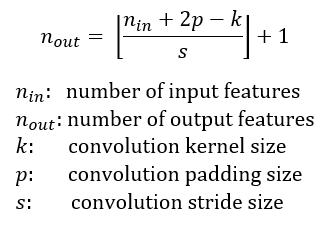
The receptive field is defined as the region in the input space that a particular CNN’s feature is looking at (i.e. be affected by). A receptive field of a feature can be fully described by its center location and its size. Figure 1 shows some receptive field examples. By applying a convolution C with kernel size k = 3x3, padding size p = 1x1, stride s = 2x2 on an input map 5x5, we will get an output feature map 3x3 (green map). Applying the same convolution on top of the 3x3 feature map, we will get a 2x2 feature map (orange map). The number of output features in each dimension can be calculated using the following formula, which is explained in detail in [1].

Figure 1: Two ways to visualize CNN feature maps. In all cases, we uses the convolution C with kernel size k = 3x3, padding size p = 1x1, stride s = 2x2. (Top row) Applying the convolution on a 5x5 input map to produce the 3x3 green feature map. (Bottom row) Applying the same convolution on top of the green feature map to produce the 2x2 orange feature map. (Left column) The common way to visualize a CNN feature map. Only looking at the feature map, we do not know where a feature is looking at (the center location of its receptive field) and how big is that region (its receptive field size). It will be impossible to keep track of the receptive field information in a deep CNN. (Right column) The fixed-sized CNN feature map visualization, where the size of each feature map is fixed, and the feature is located at the center of its receptive field.

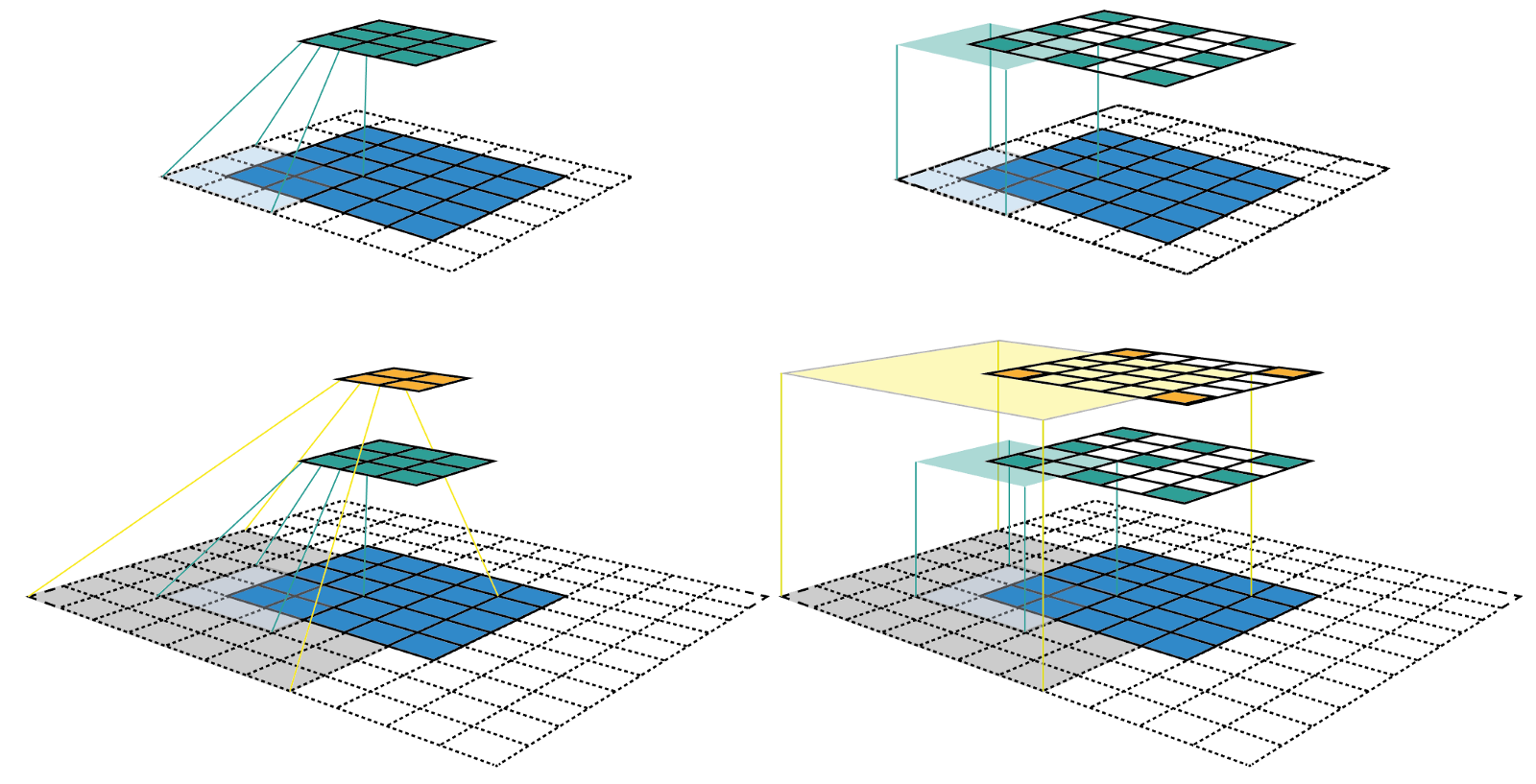
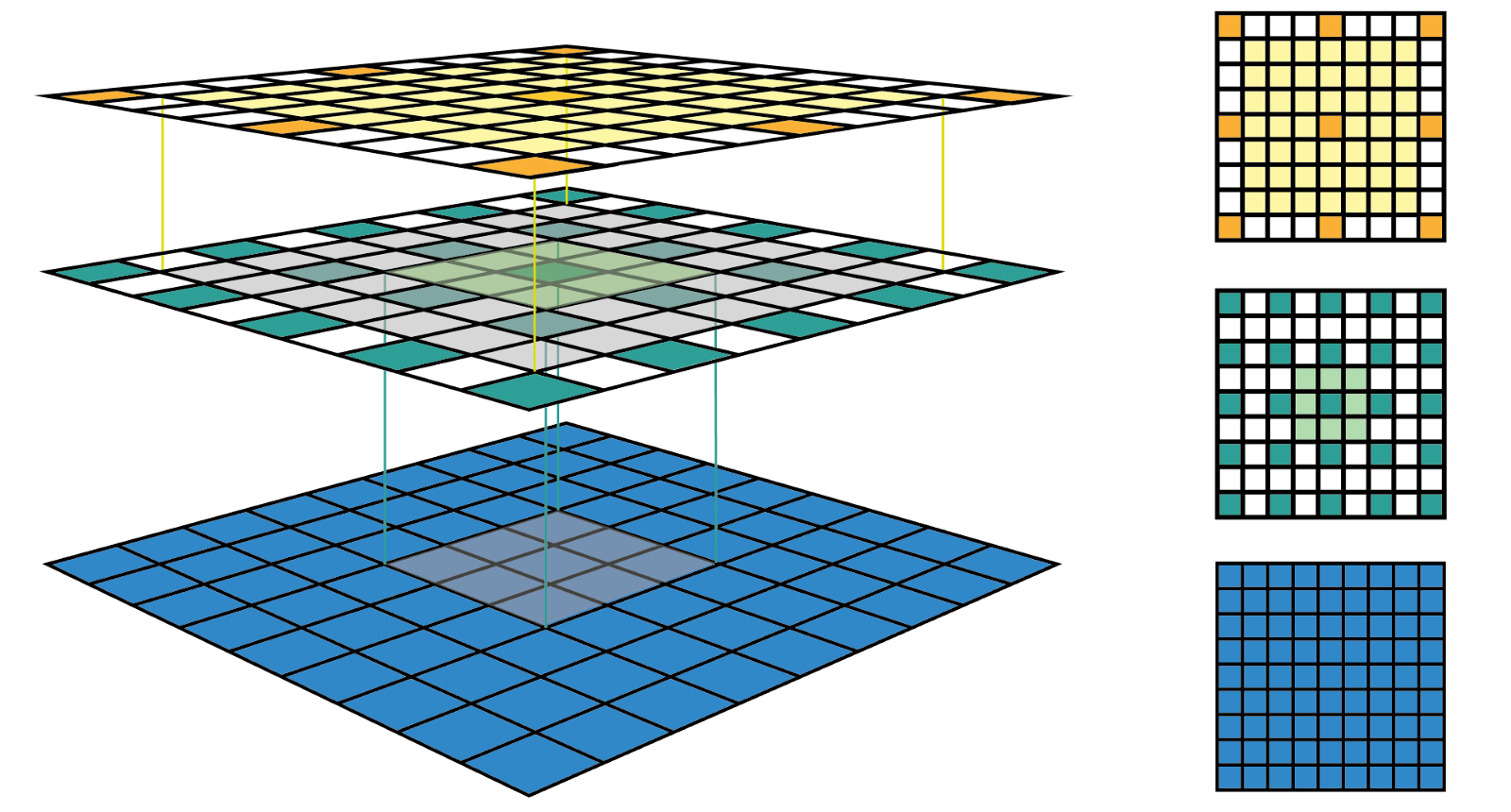
The left column of Figure 1 shows a common way to visualize a CNN feature map. In that visualization, although by looking at a feature map, we know how many features it contains. It is impossible to know where each feature is looking at (the center location of its receptive field) and how big is that region (its receptive field size). The right column of Figure 1 shows the fixed-sized CNN visualization, which solves the problem by keeping the size of all feature maps constant and equal to the input map. Each feature is then marked at the center of its receptive field location. Because all features in a feature map have the same receptive field size, we can simply draw a bounding box around one feature to represent its receptive field size. We don’t have to map this bounding box all the way down to the input layer since the feature map is already represented in the same size of the input layer. Figure 2 shows another example using the same convolution but applied on a bigger input map — 7x7. We can either plot the fixed-sized CNN feature maps in 3D (Left) or in 2D (Right). Notice that the size of the receptive field in Figure 2 escalates very quickly to the point that the receptive field of the center feature of the second feature layer covers almost the whole input map. This is an important insight which was used to improve the design of a deep CNN.

Figure 2: Another fixed-sized CNN feature map representation. The same convolution C is applied on a bigger input map with i = 7x7. I drew the receptive field bounding box around the center feature and removed the padding grid for a clearer view. The fixed-sized CNN feature map can be presented in 3D (Left) or 2D (Right).

Receptive Field Arithmetic

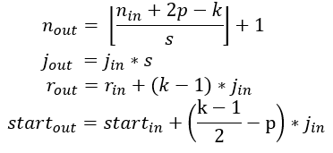
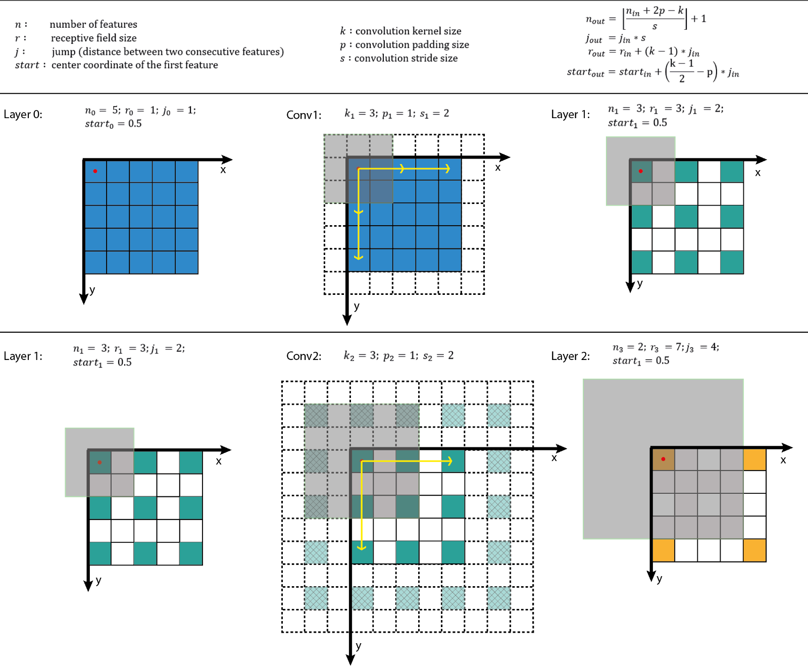
To calculate the receptive field in each layer, besides the number of features n in each dimension, we need to keep track of some extra information for each layer. These include the current receptive field size r, the distance between two adjacent features (or jump) j, and the center coordinate of the first feature (start). When applying a convolution with the kernel size k, the padding size p, and the stride size s, the attributes of the output layer can be calculated by the following equations:

The first equation calculates the number of output futures based on the number of input features and the convolution properties. This is the same equation presented in [1].

The second equation calculates the jump in the output feature map, which is equal to the jump in the input map times the number of input features that you jump over when applying the convolution (the stride size).

The third equation calculates the receptive field size of the output feature map, which is equal to the area that covered by k input features (k-1)*j_in plus the extra area that covered by the receptive field of the input feature that on the border.

The fourth equation calculates the center position of the receptive field of the first output feature, which is equal to the center position of the first input feature plus the distance from the location of the first input feature to the center of the first convolution (k-1)/2*j_in minus the padding space p*j_in. Note that we need to multiply with the jump of the input feature map in both cases to get the actual distance/space.

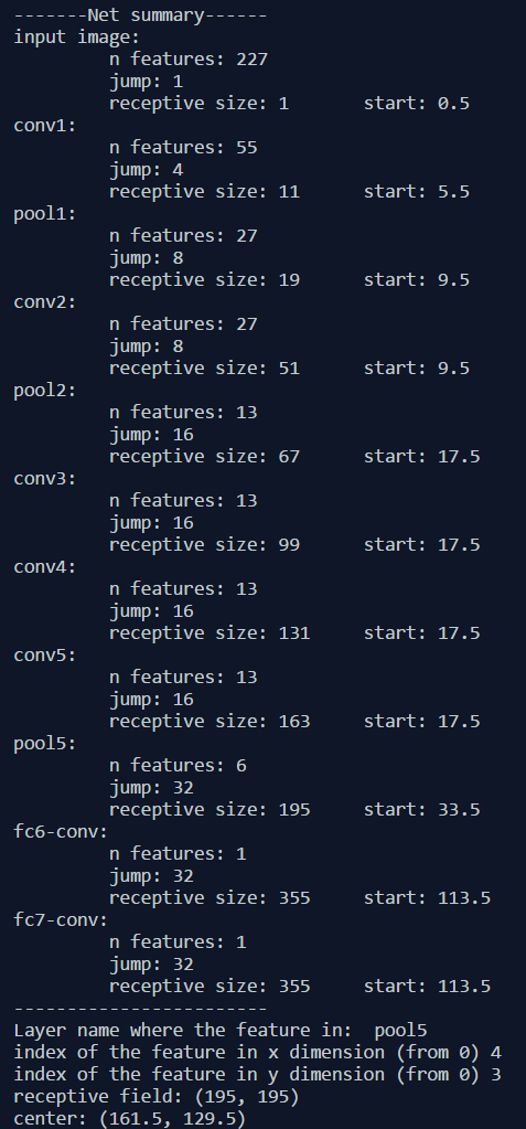
The first layer is the input layer, which always has n = image size, r = 1, j = 1, and start = 0.5. Note that in Figure 3, I used the coordinate system in which the center of the first feature of the input layer is at 0.5. By applying the four above equations recursively, we can calculate the receptive field information for all feature maps in a CNN. Figure 3 shows an example of how these equations work.

Figure 3: Applying the receptive field calculation on the example given in Figure 1. The first row shows the notations and general equations, while the second and the last row shows the process of applying it to calculate the receptive field of the output layer given the input layer information.

I’ve also created a small python program that calculates the receptive field information for all layers in a given CNN architecture. It also allows you to input the name of any feature map and the index of a feature in that map, and returns the size and location of the corresponding receptive field. The following figure shows an output example when we use the AlexNet. The code is provided at the end of this post.